Particle response to Low Reynolds Number
Oscillation of a Fluid in Microgravity
Drew L’Espérance*, Jim Trolinger†, Roger Rangel‡, and Carlos Coimbra§
This paper presents an experimental study of the response of a particle to the movement of a fluid in which it is suspended. The equations governing the motion of particles in the low Reynolds number regime have recently been solved analytically, and the solutions were used to design experiments to measure the most evasive term in the equation, known as the Basset history force. The objectives of the study are to compare experimental results with the solution to the particle equation of motion. Since the movement of a spherical particle in response to the surrounding fluid is predicted by the analytical solution to the theoretical equation of motion, the theory is tested by measuring the response of the particle to the fluid motion, specifically, the ratio of the particle to fluid displacement. In the experiment, particles are suspended in a fluid-filled cell, which is shaken in a carefully controlled oscillatory fashion. The particle and cell locations at the limits of motion are measured with great precision by applying electronic holography. Ground experiments were run with tethered particles to counteract gravity. The measured particle responses closely match the theoretical predictions for the full solution, and are clearly different from the solution where the history force is neglected. The results are important because they represent one of the first quantitative observations and analyses of the history force.
Introduction
In this paper, we present an experimental study of the fundamental physics of how a particle responds to the movement of a fluid in which it is suspended. This problem is relevant to many applications ranging from crystal growth in microgravity environments to particle dispersion in turbulent flows. The work is in support of a planned space-flight project, SHIVA (Spaceflight Holography Investigation in a Virtual Apparatus). The equations governing the motion of particles in the low Reynolds number regime were solved analytically only recently. Among the various predictions that can be made, the solutions have helped us design experiments that have produced a better understanding of the significance of the most evasive term in the equation, known as the Basset history force. Relevant experiments on earth where gravity dominates the equation, especially those where effects of the history force can be observed, are extremely difficult to conduct. The objectives of the ground-based study presented in this paper are to compare experimental results with the solution to the particle equation of motion and to provide support to a planned space-flight microgravity experiment where the equation of motion can be more fully tested.
This paper shows how we used both experiment and theory to identify and resolve critical issues and produce an optimal experiment design that exploits microgravity for the study. We examined the response of heavy and light particles to fluid oscillation at frequencies where the Basset history force was dominant. The particle sizes and velocities used corresponded to a low particle Reynolds number regime (Rep <1). To observe some of the interesting effects predicted by the new solutions requires the precise location of the position of a particle in three dimensions. To this end, we have developed digital holography algorithms that enable particle position location to a small fraction of a pixel in a CCD array. The experiments have provided a definitive, quantitative observation of the Basset history force over a wide range of conditions.
Background
Tchen (1947) derived a Lagrangian equation of motion for a spherical particle freely moving in a uniform, time dependent background flow as a culmination of previous work attributed to Boussinesq (1885), Basset (1888), and Oseen (1927). Coimbra and Rangel (1998) recognized that Tchen’s equation could be written in terms of fractional derivatives, and used fractional calculus to solve Tchen's equation for a generic forcing function that included both gravitational and fluid acceleration contributions. In the absence of gravity, Tchen's equation is reduced to,
![]() (1)
(1)
where D is the time-derivative operator,
a is the ratio of the fluid density to the particle
density, and ![]() =
a /(2+a ). Time is
made dimensionless by defining a particle characteristic time
t p given by 2a2/9a
n , where a is the particle radius and
n is the kinematic viscosity of the fluid. For a
freely moving particle, the fluid velocity u, particle velocity v,
and relative velocity w = v– u are rendered dimensionless by
dividing them by the characteristic velocity W0.
=
a /(2+a ). Time is
made dimensionless by defining a particle characteristic time
t p given by 2a2/9a
n , where a is the particle radius and
n is the kinematic viscosity of the fluid. For a
freely moving particle, the fluid velocity u, particle velocity v,
and relative velocity w = v– u are rendered dimensionless by
dividing them by the characteristic velocity W0.
The first term in eq. (1) is proportional to the particle acceleration, the third term in eq. (1) is proportional to the particle velocity, while the second (half-derivative) term depends upon both the velocity and the acceleration. Prior to 1998, the second term of the equation, which is the dimensionless Basset history drag, had been expressed in integral form, and thus was responsible for the integro-differential nature of the particle equation of motion. Because an integro-differential equation is typically much more difficult to treat theoretically than an ordinary differential equation, the history drag has been neglected in the majority of past particle motion studies.
Particle motion in oscillating flows has generated a significant amount of research activity. One practical example of particle motion in oscillating flows is that of a crystal suspended in a fluid subject to mechanical vibration. In sinusoidally oscillating flows, neither the particle velocity nor the particle acceleration reaches a steady state value, and all three terms on the left side of eq. (1) affect the particle motion. Coimbra and Rangel applied the general solution of Tchen's equation derived in reference to the case of a sinusoidal background flow given by u = Aeiw t, where the particle responds with a velocity v = Beiw t. A and B are complex numbers, reflecting the fact that there is generally a phase difference between the particle velocity and the background flow. The ratio of the particle velocity amplitude to the fluid velocity amplitude, h , is given by eq. (2).
![]() (2)
(2)
S is defined as the dimensionless frequency, which is proportional to the angular frequency, W , of the fluid.
![]() (3)
(3)
The ratio of velocity amplitudes is equal to the ratio of displacement amplitudes. The last term in the denominator of eq. (2) (i.e., the term proportional to Ö S) is due to the history drag, and is the dominant term when S » 1.
Experiments
Since the movement of a spherical particle in response to the surrounding fluid is predicted by eq. 2, we tested the theory by measuring the response of the particle to the fluid motion. Specifically, we measured the ratio of the particle (Ap) to fluid cell (Ac) displacement amplitudes at different forcing frequencies. The particle and cell displacements were measured by recording two in-line holograms at the extremes of the cell displacement. Because there is generally a small phase difference (
Df) between the particle motion and the fluid motion, the measured particle displacement (![]() (4)
(4)
The investigation focused on particles in fluids oscillating at dimensionless frequencies S between 0.1 and 6, where the history drag is dominant, moving at particle Reynolds numbers less than 1.
Particles and Fluid Cell
The properties of the particles and fluids used in the experiment are given in Table 1. Krytox (perfluoro-alkylether) and mineral oil were used as fluids in the experiment because they are transparent and have low flammability, low toxicity, and high viscosity. In order to test the influence of the particle to fluid density ratio on particle motion, two different cases were examined: a light particle (polypropylene in Krytox, a =2.1), and a heavy particle (brass in mineral oil, a = 0.1).
Table 1: Material properties
|
Material |
Density (g/cm3) |
Viscosity (cm2/s) |
|
krytox |
1.91 |
0.40 |
|
mineral oil |
0.86 |
1.85 |
|
polypropylene |
0.91 |
|
|
brass |
8.67 |
The ground experiments were designed to simulate a planned future spaceflight experiment using compact equipment. Since particles are expected to interact with walls that are less than 10 radii away, a small fluid cell dictates that small particles be used. The spherical particles had radii ranging 1.0 to 2.0 mm, and were suspended in the center of a cubic fluid cell with 4-cm edges.
Two windows on opposing faces of the cell provided optical access. In several experiments, an additional wall was placed in the center of the cell near the particle to examine the effects of interaction between the particle and the wall. The cell was sealed to ensure solid body motion of the fluid in the far field and to eliminate air bubbles, since movement of gas-liquid surfaces generates currents within the liquid. Several tests of the apparatus showed that oscillations of the cell did not produce currents, thus ensuring that motion of the fluid was equivalent to that of the cell.
To prevent the particles from floating or sinking, 2-cm long tethers were used to anchor the particles to either the bottom or top of the cell. Although the tethers were necessary for doing ground experiments, an unfortunate consequence of the tethers was that the tether drag sometimes affected the particle motion. We tested several different tether materials including human hair, spider web filaments, and thin nylon thread before identifying 19-m m diameter copper wire as the best choice for a tether in our experiments.
Test Cell and Shaker
In Krytox, the frequencies corresponding to S =1 are 57.3 Hz for a =1-mm particles and 14.3 Hz for a =2-mm particles. In mineral oil, which is more viscous, the frequency corresponding to S =1 is 66.2 Hz for an a =2.0-mm particle. The shaker system, shown in Figure 1, was designed to shake the cell at frequencies close to these target values. An electromagnetic voice coil actuator oscillates the cell in a sinusoidal motion with single mode frequencies from 10 to 80 Hz at amplitudes ranging between 75 and 200 m m. The cell was mounted on a single-axis traverse to constrain the vibration along a single direction. Two counteracting springs were used to center the transverse.
The recoil from the motion of the test cell was significant and was found to cause severe vibration of the experimental platform and optics when the voice coil magnets were mounted directly to the experimental platform. To absorb the recoil, the magnets were held within a brass counter-mass block mounted on a second traverse; the total mass of the counter-mass plus magnets is approximately 13 times that of the test cell plus voice coil.
A phonograph needle in contact with the cell registered the cell velocity. Motion of the needle flexed a piezoelectric crystal, producing a voltage that was proportional to velocity. A spectrum analysis of the velocity signals at the frequencies used in the experiment showed that almost all of the cell oscillation was at the fundamental frequency with very little distortion. Distortion was comprised mainly of second and third harmonics of the fundamental mode, which were at least three hundred times less intense than the fundamental mode in our experiments
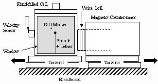
Figure 1. Diagram of the electromagnetic shaker.
Measurement Techniques
The optical layout of the experiment is shown in Figure 2.
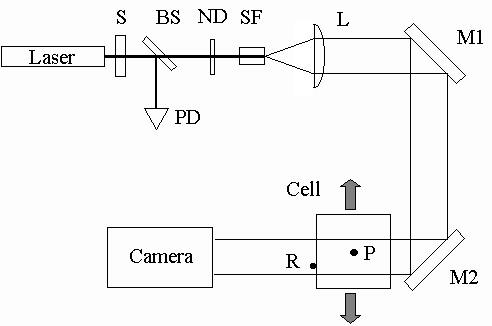
Figure 2. Optical Layout of Experiment
The illumination source was a 10 mW HeNe laser that was modulated by a shutter (S). A beam-splitter (BS) diverted a small amount of the light into a photodiode (PD); this signal was used to monitor the opening of the shutter. The illumination intensity was adjusted by a neutral density filter (ND), then spatially filtered (SF) and collimated by a lens (L). Two mirrors (M1 and M2) aimed the defocused beam at normal incidence through the cell, which oscillated horizontally. A 0.5-mm radius sphere (R) was glued to the back window of the cell to serve as a cell reference marker, and the particle (P) was inside the fluid-filled cell.
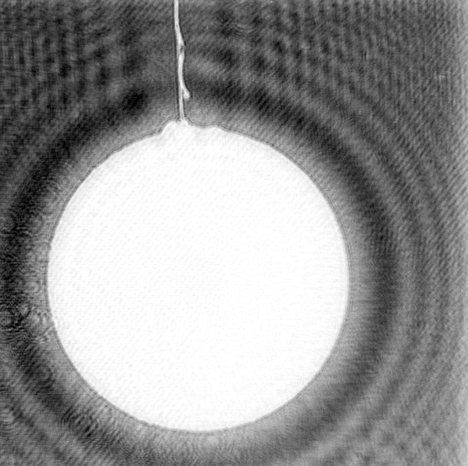
In-line holograms of the shadow of the particle and reference marker were recorded using a 1024 x 1024 pixel Kodak MegaPlus ES 1.0 CCD camera with no lens located between 10 and 20 cm behind the cell. The pixels were 9m m squares. The shutter was triggered to open for 0.8 ms at the two extremes of a cell oscillation cycle when the cell velocity was zero. The camera was operated in double-exposure mode and synchronized with the shutter, resulting in two images of the cell at the two extremes of cell motion. This method is relatively insensitive to low-frequency vibrations that cause the center position to drift. A sample in-line hologram is shown in Figure 3.
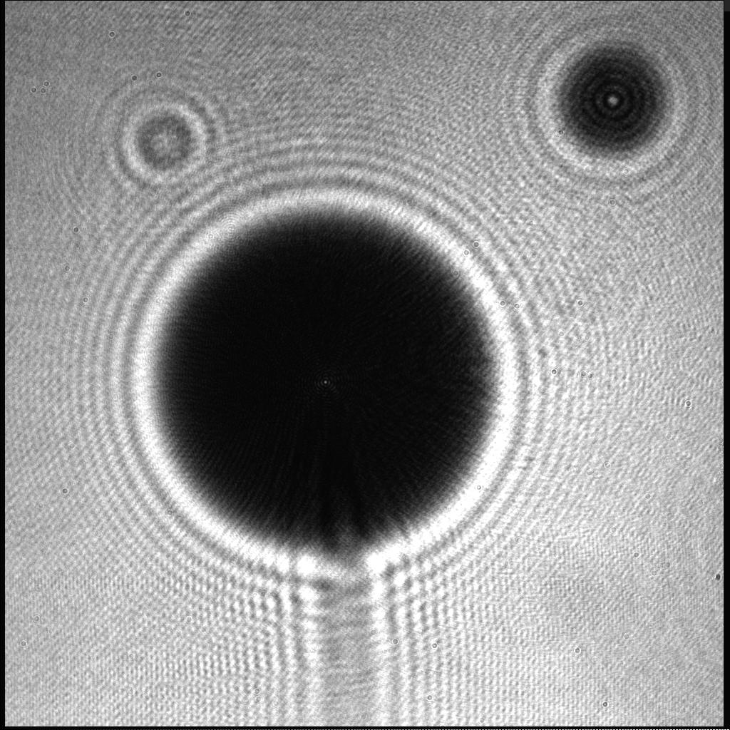
Figure 3. In-line hologram of a 2-mm radius particle (large circle in center of photo). The tether is attached to the bottom of the particle. The smaller circle in the upper right corner is the cell marker.
Measuring the cell and particle position
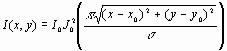
The position of the cell and particle were determined from the in-line holograms by cross-correlating the holograms with an analytically generated template. This method relies on the fact that the Fresnel diffraction pattern from a spherical object can be computed given the radius of the sphere a, the distance between the object and camera z, and the wavelength of light l . The bright spot at the center of the diffraction pattern (known as Poisson’s spot) and the surrounding rings provide an excellent noise free, predictable light pattern that is used as a correlation template. For the region of the shadow within half a radius of the center, the intensity I(x, y) of a pixel with coordinates (x, y) is approximated by eq. 5,
 (5)
(5)
where I0 is the intensity of the center of the Poisson spot, J0 is the zeroth order Bessel function, x0, y0 are the coordinates of the pattern center, and s is the ring spacing in pixels. The ring spacing depends upon the particle radius a, the distance between the camera and particle z, the wavelength of light used l , and the length of each pixel s (eq. 6).
![]() (6)
(6)
The ring spacing of the particle was computed by locating the brightest pixel in the center of the particle shadow, calculating the average radial intensity distribution I(r) centered on this pixel, then using the Levenberg-Marquardt method to find the best fit of eq. (5) to the radial intensity distribution with I0 and s as adjustable parameters (see Figure 4). The same method was used to find the ring spacing of the cell marker.
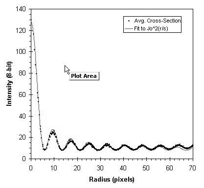
Figure 4. Plot of experimental radial distribution function [I(r) vs. r] centered on Poisson spot. The radial distribution function is fit by I0J2(r/
s) to determine the ring spacing, s .Once the ring spacing of the particle and cell marker were determined, a template image was generated in the form of eq. (5). The size of the template was limited to approximately the region within half the radius of the particle or cell marker. Ideally, the template represents the pattern of rings as it would appear if the noise, which is not circularly symmetric, were averaged out.
During a typical experiment, batches of 70 or more images of a single tethered particle were recorded, all having the same ring spacing. Therefore, we determined the average ring spacing for four sample images, generated the template corresponding to this ring spacing, and used the template to analyze every image in the batch. The images were analyzed by extracting a square region of interest near the center of the particle shadow to make a source image equal in size to the template, then computing the cross-correlation (X) of the source (S) and template (T) according to eq. (7),
![]() (7)
(7)
where Á and Á -1 represent the Fast Fourier Transform and Inverse Fast Fourier Transform operators, respectively.
The maximum of the cross-correlation (see Figure 5) corresponds to the position where the template best overlaps the source image, and should also correspond to the true center of the particle.
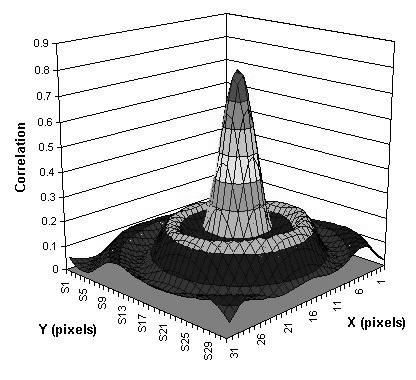
Figure 5. Surface plot of the cross-correlation function. Only the 1024 pixels at the center of the array are shown. The surface elevation represents the intensity of the correlation function.
The particle and cell positions or amplitudes must be determined with an accuracy of 5 microns. It would be beneficial to do better than this, say 1 to 2 microns. Since the pixels are 9 m m in length, we developed an interpolation procedure to locate the cross-correlation peak to sub-pixel resolution. The procedure extracts two 5-pixel arrays, one vertical and the other horizontal, centered about the pixel with the maximum correlation value. The correlation intensities of each five-pixel array were then plotted versus position and fit by a parabola. The vertices of the parabola correspond to the coordinates of the cross-correlation peak (see Figure 6).

Figure 6. To locate the correlation peak to sub-pixel accuracy, two 5-pixel arrays centered on the maximum (one horizontal and the other vertical) are extracted from the cross-correlation. Each array is fit by a parabola, giving the coordinates of the cross-correlation peak to 0.1-pixel resolution.
We tested the program by constructing synthetic images of a particle upon a noisy background, where the particle center was known. The program was able to locate the center of the particles to within 0.1 pixel or better. In another test, we used a micrometer to displace a fixed particle by amounts ranging from 88 to 108 m m. Comparison between the mechanically measured and optically measured displacement confirmed that the particle could be located to a precision of at least 0.1 pixel, or 1 m m.
Results
Figure 7
shows a plot of the experimentally measured particle response Re(h ) versus dimension-less frequency for two different polypropylene particles in krytox (a =2.1), one with a radius of 1.00 mm and the other with a radius of 1.98-mm.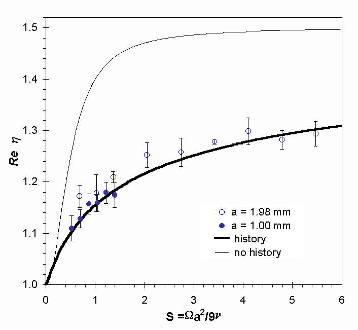
Figure 7. Plot of Re(
h) vs. S for polypropylene particles in Krytox (a =2.1).Figure 8 shows a plot of Re(h ) versus S for three different radii (1.00, 1.59, and 1.98-mm) brass particles in mineral oil (a =0.1). The uncertainty bars in both figures represent the 95% confidence limit. Also shown on both figures are the theoretically predicted response curves with the history term included (bold curves) and neglected (thin curves). In both cases, the data closely match the theoretically predicted response curve where history effects are included, and the experimental uncertainty is much less than the difference between the two curves.
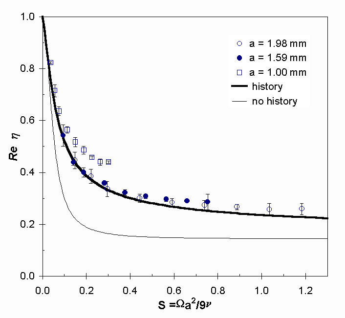
Figure 8. Plot of Re(
h) vs. S for brass particles in mineral oil (a =0.1). The theoretical curve closely matches the data except for the smallest particle (a =1.00-mm) and the two heavy particles at high frequencies.Particle Motion at Particle Reynolds number > 1
We investigated the effect of particle Reynolds number on the response of heavy particles to cell motion by examining a 1.98-mm radius brass sphere in krytox (a =0.22). The experiments were carried out at a cell oscillation frequency of 14.9 Hz, at which frequency the dimensionless frequency S = 1.02. The particle Reynolds number was varied by adjusting the cell amplitude (Ac); the particle Reynolds number can be determined from the cell amplitude and magnitude of the displacement ratio, according to eq. (6).
Rep = 9SAc(1-|h |)/a (6)
For this part of the investigation, we collected a series of images at different phases of the cell motion so that Ap, Ac, h , and
Df could be measured directly. This was accomplished by leaving the shutter open, setting the camera exposure time to 0.1 ms, and triggering the camera by a pulse generator synchronized to the voice coil driver signal. A series of 75 images were recorded at 3 s intervals with the delay between the driver signal and the trigger pulse varied between images; the delay was typically varied over a range covering two periods of the cell oscillation. The disadvantage of this triggering method is that the images are collected over a relatively long time (about 3 minutes), so the measured cell and particle positions must be corrected to account for small low-frequency vibrations that cause the cell zero position to drift. Figure 9 shows a sample plot of the particle and cell position versus delay time.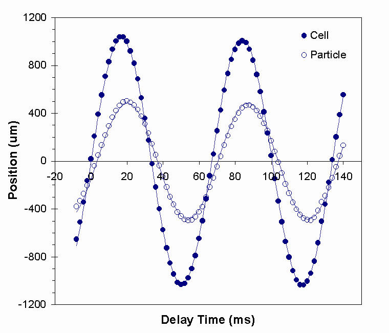
Figure 9. Plot of cell and particle position vs. delay time for an a=1.98 mm brass particle in krytox (a =0.22) oscillating at 14.9 Hz (S=1.02). The positions of the test cell and particle were fit by sine waves to determine Ap, Ac, and
Df.The results for oscillation of the brass particle at 4 different particle Reynolds numbers are given in Table 2. The results show that |h | and
Df are nearly constant over particle Reynolds numbers ranging from 0.8 to 3.2. The results are very close to the theoretically predicted values for S =1.02 and a =0.22 at low Reynolds number, which are |h | =0.474 and D f = -17° . If history effects are neglected, the theory predicts |h | = 0.311 and D f =-12.5° .Table 2. Results from a=1.98-mm brass particle in krytox (a =0.22) oscillating at 14.9 Hz (S = 1.02) at different particle Reynolds numbers.
|
Ac (m m) |
Rep |
|h| |
Df |
|
317 |
0.78 |
0.471 |
-19° |
|
636 |
1.56 |
0.471 |
-19° |
|
907 |
2.22 |
0.473 |
-19° |
|
1322 |
3.23 |
0.474 |
-19° |
We performed virtually the same experiment with a 1.98-mm polypropylene particle in Krytox (a =2.1) with Rep ranging from 0.14 to 1.06. The results are presented in Table 3. Once again, the values of |
h| and Df are nearly constant over the Rep range, and are close to the theoretically predicted values with history included (|h| = 1.170 and Df = +6.1° ), but very different from the predicted values where history is neglected (|h| = 1.443 and Df = +8.5° ).Table 3. Results from a=1.98-mm polypropylene particle in krytox (a =2.1) oscillating at 14.9 Hz (S = 1.02) at different particle Reynolds numbers.
|
Ac (m m) |
Rep |
|h| |
Df |
|
181 |
0.14 |
1.170 |
+6.4° |
|
375 |
0.30 |
1.173 |
+6.4° |
|
524 |
0.41 |
1.170 |
+6.4° |
|
782 |
0.62 |
1.170 |
+6.4° |
|
1060 |
0.84 |
1.170 |
+6.4° |
|
1347 |
1.06 |
1.169 |
+6.4° |
Tether effects.
In order to examine the effects of tethers on the particle motion more closely, we reconstructed images from the in-line holograms. The digital reconstruction process is described in reference . Two reconstructions of a tethered 1.98-mm radius brass particle, one taken at the left extreme of particle motion and the other at the right extreme, are shown in Figure 10. The images show that as the particle moves, it pivots about the tether attachment point. The result is that the particle rotates about 10° while the tether swings through an angle of about 3° . The effect is especially noticeable when the series of images are animated.
 |
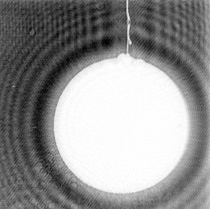 |
| a) near left extreme | b) near right extreme |
|
Figure 10. Negative reconstructed image of an a =1.98 mm tethered brass particle in krytox at two extreme positions. The particle pivots about the tether attachment point. |
|
The pivoting motion of the particle may explain some of the discrepancies between the experimental data from brass particles and the theoretical curves seen in Figure 8. For all three particles, the difference between the experimental data and the theoretical curves increases as the cell frequency increases. Since the velocity of the particle is proportional to the cell frequency, increasing the oscillation frequency increases the particle velocity for a fixed amplitude. The pivoting motion of the particle should increase as the particle velocity increases. Furthermore, the greatest difference between the experimental data and the theoretical curves occurs for the smallest particle size (a =1-mm). The small particles may be more affected by the pivoting motion because their mass is much less than the other particles. We did not observe this tether effect in our experiments with tethered polypropylene particles.
Conclusions
In the foregoing, we have presented some results of a ground based experimental program that is designed to support the flight experiment SHIVA. Using a tethered particle method to simulate microgravity, we conducted a range of experiments, identified and resolved what appear as the most challenging obstacles to a successful experiment, and have developed the necessary methods to meet experiment goals.
The results show that the tethered particle method is a viable experimental method for ground experiments, and the data are largely consistent with theoretical predictions provided that the particles are not too small. The results also suggest that Tchen’s equation may also apply for particle Reynolds numbers up to 3. However, experiments with tethered particles at high Reynolds numbers should be interpreted cautiously. Trends that appear to follow the particle Reynolds number may in fact be due to tether effects.
Acknowledgements
This work is supported by NASA’s flight definition project SHIVA (Spaceflight Holography Investigation in a Virtual Apparatus) under contract number NAS8-98091. The NASA management team includes M.Bodiford, Project Manager, Dr. D. Smith, Project Scientist, W. Patterson, Systems Engineer, all from NASA’s MSFC. The authors wish to acknowledge M. Dempsey of MetroLaser for conducting much of the experimental work.
REFERENCES