TECHNIQUE FOR SIMULATING AND EVALUATING
AERO-OPTICAL EFFECTS IN OPTICAL SYSTEMS
J.D. Trolinger, MetroLaser Incorporated, Irvine, CA
W.C. Rose, Rose Engineering and Research, Reno, NV
Abstract
This paper describes a new computer model and code for simulating aero-optical effects on light propagation through an aerodynamic flow field. The code exploits the ability of computers to easily mimic random media and simulate the optical effects of turbulent boundary and shear layers. This enables optical propagation experiments through all kinds of random optical media to be performed in the computer. The resultant aero-optics computational test simulator (AOTS) allows a designer to simulate and run aero-optical tests that will be useful for system evaluation, test planning and data interpretation.
Background
Aero-optics is the science that deals with (usually unwanted) effects on an electromagnetic wavefront caused by aerodynamics. These wavefront effects are caused by refractive index variations that occur in aerodynamic flow fields and distort the wavefront by delaying or advancing parts of it by different amounts. For most gases, index-of-refraction fluctuations are proportional to the fluid density fluctuations through the Gladstone-Dale constant.
Many types of optical systems (i.e., designators, rangers, LIDAR, laser communicators, directed energy weapons) receive or project light through an aerodynamic flow field, which effectively inserts an unwanted, time-varying, optical element into the system leading to loss of resolution, bore sight error, tracking error, reduction in signal to noise, and reduced energy density on a target. The capability of almost all of these devices is deteriorated by aero-optical effects on the optical wavefront caused by flow features of the aircraft, such as shear and boundary layers. These problems have been observed in many flight and wind tunnel tests since the early years of testing of USAF airborne lasers.,
Many attempts to understand and solve the aero-optics problem have been made with limited success for parts of the problem.,. These include attempts to minimize aero-optical effects, as well as correcting for them. In general, the problem requires a multidisciplinary approach that marries aerodynamics and optics, including experimental and computational capabilities in both the optics and aerodynamics of turbulent flow. Developing and testing solutions require experimental simulation facilities (e.g., wind tunnels) and optical diagnostic tools are needed to quantify both the simulation and the solutions. Computational simulations and tests can be extremely useful in designing and interpreting experimental test results. This paper focuses on the latter.
Computational simulations of aero-optical phenomena can play a vital, complementary role in complete system design, analysis, test planning, and test data interpretation. The present work addresses the need for improved aero-optical effects simulation to augment system test planning and data interpretation.
To simulate the effects of aero-optic phenomena on the wavefront, the computer model incorporates a set of time varying (in general) phase screens that are derived from physically meaningful models. By using a combination of experimental data and CFD, screens can be created that emulate real-world conditions. Each screen is positioned within the model’s coordinate system at the appropriate location and orientation relative to the imaging system and simulates a single, specific aero-optic phenomenon. The simulator then projects light waves through the modeled space as it develops in time, producing realizations for a large number of frozen instances on a time scale that is known to be appropriate for each phenomenon. The final time resolved effect at the image plane is then determined by appropriately analyzing, sampling and averaging the realizations.
Aero Optics Code
Many attempts have been made to model and predict the optical effects of propagation through random media, using CFD as well as various turbulence models. Most available results are difficult to apply to practical problems, especially problems in aero optics. Recognizing that random media are relatively easy to set up computationally with algorithms that can mimic turbulent boundary and shear layers, we designed an algorithm that complements and is integrated with CFD. This allows us to include high frequency effects that are not accommodated in current CFD codes. The resulting code allows us to conduct simulated propagation experiments in a much wider range of realistic flows.
The MetroLaser aero-optics code assumes that the entire optical path from source to sensor can be divided into regions that are each characterized by a refractive index distribution, which can be further represented optically by a single-phase screen that is positioned appropriately in the region of space that it represents. Once the phase screens and their locations are defined, an optical wave is propagated through the set of phase screens using the optics code ZEMAX to determine the net effect on the wavefront at the sensor.
We assume that the phase screens that are sufficiently weak will not be overly sensitive to location along the optical path. This simply means that the rays of light are refracted only at small angles, an assumption that is largely true in air. The phase screens are defined and derived in such a way that various flow conditions and model parameters can be easily changed, so that computer experiments can be run to cover many different experiment types. The goal is to provide a tool that can assess the importance of individual regions and parameters, and act as an aid in test planning and evaluation.
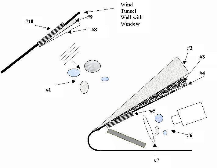
For example, a typical aero-optical wind tunnel test includes the following: turbulent boundary layers over wind tunnel windows, wind tunnel free stream, shock wave, coolant and shear layer, model boundary layer, window distortion, internal flow, and internal optics. The AOTS creates a phase screen (or possibly more than one) to represent each region. Each phase screen is produced from an appropriate optical model of the region that, for some cases, incorporates information provided by CFD.
The phase screen modules represent the regions shown in detail in Figure 1. They are:
1. Free stream turbulence (or, in the case of a flight vehicle, the atmospheric turbulence).
2. The shock wave.
3. A shear layer, caused by a coolant.
4. A turbulent boundary layer.
5. A window that is distorted by thermal gradients and mounting stress.
6. Internal turbulent air in the seeker body.
7. The seeker optics.
8. A shock wave on the opposite wind tunnel window.
9. A turbulent boundary layer on the wind tunnel window.
10. A window distorted by thermal and mounting stresses.
Creating Phase Screens
Turbulent Layers — The phase screens for turbulent layers are generated from a logical, realistic representation of a turbulent flow. If the full three-dimensional, time-resolved density distribution could be computed, then the refractive index field would be known and a time-dependent phase screen containing even the turbulence could be computed directly. While CFD may be able to provide useful computations for achieving portions of this, it is impractical to resolve fully the required small-scale flow properties, especially at high turbulent frequencies. Our model supplements CFD by an ad hoc modeling of these small-scale properties. This is equivalent to sub-grid modeling.
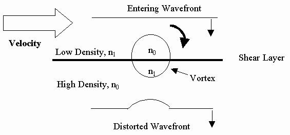
To proceed in our desire to model the full optical path, we have devised and tested a variety of other methods to complement CFD. The chosen model (see Figure 2) depicts turbulence as a random distribution of spheres of gas with a change in refractive index/density from the surrounding region, both positive and negative. These result as vortices move gas from a higher (lower) density to a region of lower (higher) density.
A larger vortex acts over a larger density gradient and, therefore, must be represented by a sphere of larger density change. In addition, spheres lying in a region of higher density gradient should be represented by a larger density change. For a linear gradient, all the spheres of one size contain a single density using this rule. Sphere sizes range from an upper diameter of the shear/ boundary-layer thickness to a lower range of 1/10 to 1/100 the dimension of the shear/boundary layer, depending on the effects that the smaller scale sizes have on the salient optical parameters.
The density changes were selected for a given frozen flow state (i.e., a snapshot) by a set of rules based on experiment and theory. The distributions of size and density differences (i.e., the fluctuating density associated with each sphere) were also selected by a set of rules (described in detail below), incorporating a random change from one frozen flow state to the next. This model is consistent with the notion of a mixing length for the turbulent flow.
The phase change caused by passing through a sphere was computed using parameters that include sphere diameter and density change. Each sphere is considered to be a weak phase object and diffraction is neglected. Therefore, the phase in a plane after the sphere is not affected by the location of the sphere, and we can lump the phase effects of a 3D distribution of spheres into a single-phase screen, as long as the distribution remains relatively thin. (A similar treatment is used in the "thin lens" equations, which model the entire phase change occurring at a plane.)
The model for a particular region of the flow, like a turbulent boundary layer, is illustrated in Figure 3. Spheres are placed randomly throughout the volume with a chosen size distribution to represent one realization (or one instant in time) of frozen flow. Then the optical path length is calculated for all rays to produce a phase screen at the bottom of the volume. The weak phase object assumption allows the rays to pass straight through the flow without bending or scattering. Therefore, the result is the same as would be obtained if all of the spheres were placed randomly in a plane with the same rules for density and size distribution being applied.
We considered various rules for the total allowed number of spheres, as well as for overlapping spheres. Since smaller eddies are known to exist within larger eddies, overlapping of smaller with larger spheres is allowed. The hierarchy of turbulent scales can be summarized by the following:
Molecular
Mean free path (mfp)
Dissipation length (10-100 mfp)
0.2
0.4
d-Shear layer (d is the shear layer thickness)1.2
d ("rollers")Each phase map for a given random set of spheres represents a snapshot of the flow at an instant and is uncorrelated with phase maps for other random sets of spheres. Such a phase map corresponds to a phase map produced experimentally by a pulsed diagnostic wavefront sensor that freezes the flow. Now if we compute a sequence of such randomly generated independent sets and add them together, we should obtain a representation of the time-averaged flow.
The following is a detailed description of the algorithms for constructing the phase screens for turbulent layers, shown graphically in Figure 4:
1. From CFD or other sources:
·
Obtain mean velocity profiles.·
Determine the turbulent layer thickness, d, in the region of interest. (Depending on how definitive the profile is, this may require judgment on the part of the user.)·
Obtain mean density profiles (and the mean density gradient).·
Determine the total change in density across the layer, D r .·
Determine the length scale, l k- w , produced by using a k-w turbulence model which we define as k1/2 /w or a representative average of k1/2 /w.2. Determine
Lr , a characteristic sphere (turbulence scale) diameter that is related to the turbulence length scale, from the following (based on empirical observations):Shear layer:
Boundary layer:
Lr= 5 l k- wOther types turbulent layers or user specified layers:
Lr is related to experimentally observed layer characteristics. Examples are:o
Free streamo
Optical traino
Atmospheric3. Choose an appropriate size probability distribution for p spheres, with the nth sphere having diameter,
Ln, that we use to model turbulence in the layer under consideration.3.1. For boundary and shear layers we select a size distribution that exponentially decreases with diameter:
P(
Ln)=Kexp(-Ln/Lr ),where
Lr is defined above.And we require
![]() P(
P(
so that
K= 1/![]() exp(-
exp(-
Place appropriate limits on the parameters as follows:
Boundary layer:
Lr=0.20 d0.01
d < L < 0.6 d,and
Pb(
Ln)=Kexp(-5Ln/d ).Shear layer:
Lr= 0.40 d0.02
d < L < 1.2 d,and
Ps(
Ln)=Kexp(-2.5Ln/d ).3.2. Another turbulent layer more representative of a wind tunnel free stream is Gaussian where:
![]()
For AEDC Tunnel 9 free stream turbulence:
We selected s = 2 mm and 1 mm
3.3. Other distributions may be required for different types of turbulent layers.
4. Create the p spheres that will be used to model the turbulence by selecting randomly from the appropriate size distribution. (A number of software programs are available to do this.) We achieve this by creating a line containing N line segments, representing N different sphere diameters that cover the allowed size range. The lengths of each of the segments are made to be integral numbers by multiplying a large number times the value of the distribution function for that diameter. Then a random number generator generates p numbers from a sample that covers the extent of all of the line segments. Each of the p numbers is associated with a specific segment and, therefore, a specific sphere diameter.
The number of spheres, p, is ultimately based on experimental observations. It is a number that can fill, or even overfill, the volume of the turbulent layer. Typical numbers used are hundreds to thousands, and fill the volume with fill factors as high as two or more.
The length of the nth line segment, which is associated with the,
Ln, is proportional to one of the following:Exponentially decreasing: P(
(Since we are interested only in the relative probability for each size, the value of the normalizing constant, K, plays no role here and can be set to 1 for simplicity.)
Gaussian: ![]()
5. Using a random number generator, generate for each of the p spheres a random xy position in the optical aperture.
6. Determine the density difference for each sized sphere from the following relationship:
For
L< Lr Dr¢ = (Dr/ d) (0.2 L),i.e., the density change is the density time the mixing length.
For
L> Lr Dr¢ = (Dr/ d) (0.2 Lr).This is considered the "fluctuating density" (it is equally probable to be positive or negative).
7. For each turbulent component of the flow, populate a slab with the p spheres at the random x and y positions in the aperture and assign alternating positive and negative values to each.
8. Compute a phase screen for each slab by calculating the optical path length through the populated (with spheres) slab. This is the integrated product of the path and refractive index of the fluid. Compute the refractive index of the fluid by using the Gladstone-Dale relationship.
D
n = GDr,The additional phase change experienced by a ray passing through a single sphere at some (x, y) location relative to the sphere’s center is determined by using the relation:
Df
= 4p Dn/l (L 2 - x2 - y2)1/2 = 4p (GDr)/l ([L /2]2 - x2 - y2)1/2,where
Df is the added phase due to the sphere, L is the sphere diameter, and Dn is the change in refractive index inside the sphere relative to the ambient condition outside the sphere.9. Position the phase screens for all components under consideration in the appropriate spatial positions as surfaces in the ZEMAX optical code input.
10. Use ZEMAX to propagate an incoming wave through all of the phase screens to a point of interest.
11. From ZEMAX solutions, at points of interest compute the desired optical characteristics, such as phase maps, Strehl ratios, point spread functions, and contained energy. This represents data from one instantaneous snapshot taken at a random time, characterizing a frozen flow field, and would simulate pulsed laser diagnostics. To determine averages and measurements of averages, statistically meaningful numbers of such data sets will be required.
12. Determine time averages and flow development by using random number generators to compute sets of phase masks, each set representing the flow field at one instant of time. From each set, compute a phase distribution at a point of interest. From averages of many sets, compute time averaged flow properties.
Time averages would represent what CW laser diagnostic measurements provide.
Shock Wave — When CFD provides the shock wave position, no additional phase screen is necessary. If shock waves are not provided by CFD, the AOTS code provides for four types of shock waves: planar, cylindrical, conical, and sinusoidal. The user must specify a density ratio, a beam direction, and a shock geometry. Plane shock waves for most practical cases do not deviate (refract) a light wave significantly. Sinusoidal shock waves can be used to represent an unsteady shock.
Windows — Windows distort a wavefront through various mechanisms that are modeled, including refractive index variations caused by temperature gradients, mechanical distortions, and optical quality. An interferogram of a window provides the phase screen that represents the window effects on the wavefront.
Steady Flow — CFD provides a distribution of density over a three-dimensional space on a grid. Required inputs are grid location equations and the density values. The AOTS code allows the user to choose an optical path through this field for beam propagation, and the aero-optical effects of the steady flow component are determined by integrating along the optical path. This leads to the phase over a surface, which becomes another phase screen to be added along with the others.
In principle, this is a very simple concept. In practice, it is not a trivial exercise, since the grids containing the discrete points of density information do not present themselves continuously along an integration path of a typical ray of light. The density must be transferred from millions of points on the grid to hundreds of straight lines (rays) of light. We developed an efficient algorithm that searches the entire grid for a beginning point on each ray for the 8 nearest points. The interpolated density is assigned to that first point on the line. The next search is confined to small distances from the initial point, limiting the number of grid points searched to an amount that is anticipated to contain the required points. By restricting the search in this way, a typical grid can be searched to provide densities along a line in fractions of a second.
The vast difference between the normal operational procedures and times involved in using CFD and the AOTS code had a major influence on the optimum way to link the codes. For example, in running the aero-optics code, the end result is available almost instantly after the parameters that define the various phase screens are provided. An operator can run experiments and test the effects of varying parameters essentially in real time.
Some of the required parameters are produced by CFD, which can have relatively large computational times, especially when run on a slower computer. Also, CFD is commonly run on a mainframe computer, so the times and places for operating CFD and AOTS will usually differ. Therefore, the most common way of using the system with CFD is to conduct each study in two parts. One CFD solution leads to many different scenarios for aero-optics.
Experiments
We have run a wide range of computer experiments in which we provide sets of flow conditions and examine wavefronts passed through the sets. We anchored the code with experimental data.
Statistical properties of such flows were examined to determine how many runs are needed to converge on a stable mean Strehl, wavefront deviation, and focus diameter. Individual realizations represent wavefront effects on pulsed lasers, averages represent effects on CW laser experiments, and time resolved realizations represent effects on such applications as laser communications.
We also examined the importance of turbulence parameters and scale size distribution. In many cases, the larger turbulent eddies cause the greatest aero-optical effects and the smaller spheres can be neglected.
Strehl ratio is a function of number of spheres. It increases with sphere number and eventually reaches a plateau after which it decreases.
Generic Turret — We conducted experiments on a case of the flow field over a generic laser nose turret 2 meters in diameter with a 60 cm aperture being run at M = 0.85 at 35,000 ft.. To simplify the CFD part of the work, we produced a two-dimensional solution from WIND about an axisymmetric body, then obtained the three-dimensional grid by rotating the solution 360 degrees about the axis of symmetry, which shows the two-dimensional density solution for this case. The turret is a one-meter radius. Using the procedure described above, we propagated light waves along various paths, as shown in Figure 5, wherein ray C is at a 45 degree angle with the axis, ray D is perpendicular to the axis, and rays B and A are parallel to the axis. Ray A is furthest from the influence of the turret and should represent the least perturbed case. 100 light rays covering the aperture represented each light wave.
As the light wave is propagated, each ray is phase delayed by the refractive index field, which is determined by the density field. This provides a phase screen for the aero-optical simulator that is defined by the 100 phase values. The phase screen is placed near the surface of the model, and the wavefront can then be completely analyzed in terms of its focusing parameters and Strehl ratio.
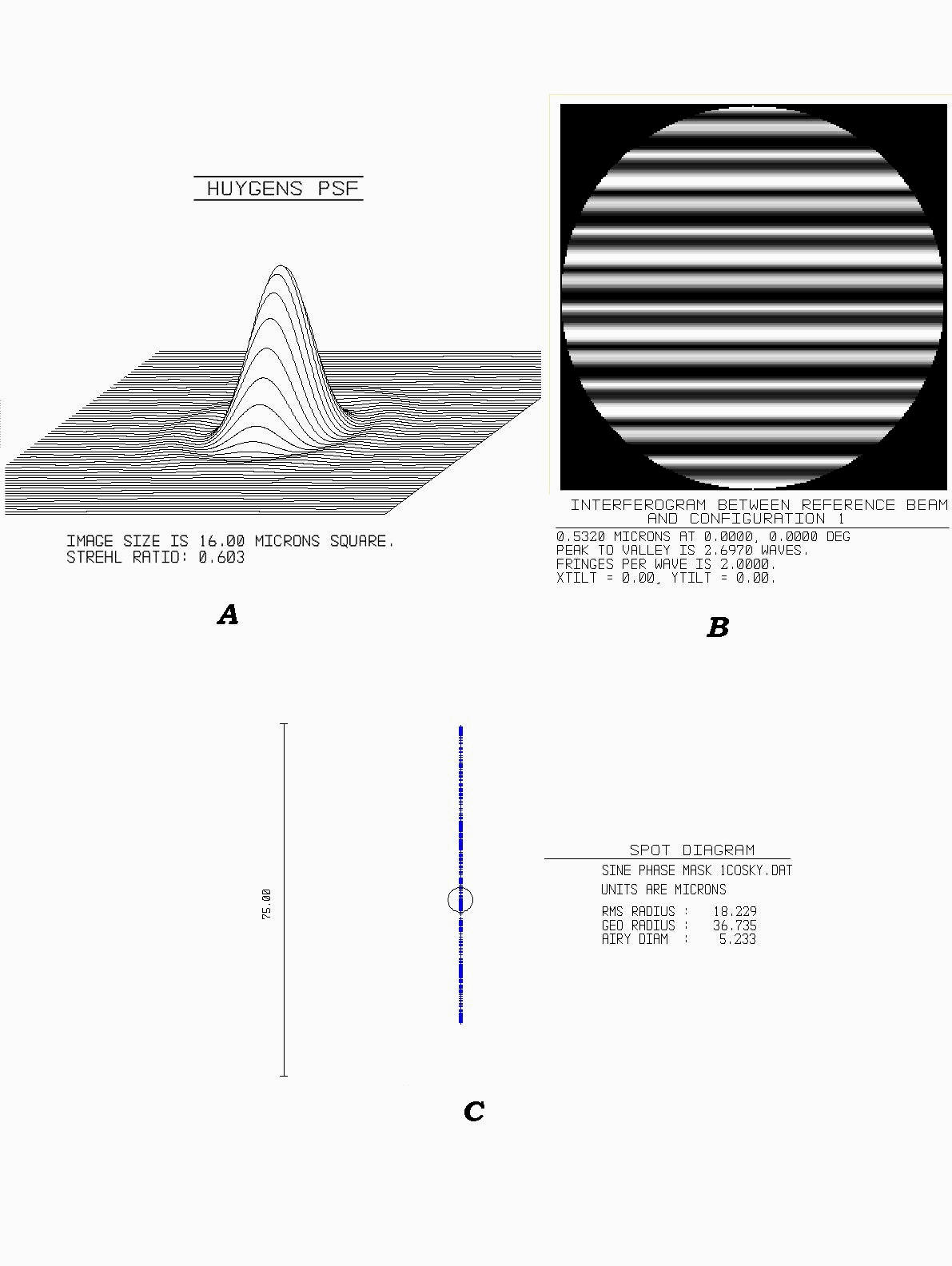
Figure 6 shows the composite end result of the beam path 10 meters above and parallel to the model using encircled energy, wavefront phase screen, point spread function, and focused spot size to display the wavefront characteristics after propagating through a computed flow condition. This is the typical output from an AOTS propagation realization. Subsequent figures are limited to the point spread function.
The path through this region is 10 meters long and fairly uniform. The upper, right-hand diagram shows the phase screen, which varies less than one wave over the aperture. There is some indication of an artifact, though it is almost negligible. There is no physical explanation of the discontinuities. These are probably the result of using a smaller number of rays to represent the wavefront. We will experiment with this to optimize this choice. The Strehl ratio is 0.86, which is relatively high, as expected. The focused spot size using ideal lenses would have a 5
μm radius, or about 10 times diffraction limited. A detail of the encircled energy plot comparing to a diffraction limited case is shown in Figure 7.Moving the wavefront down farther into the flow field causes much more severe wavefront deterioration, as we can see in Figure 8. For the next study case, a segment parallel to the model at a height of 5 meters was introduced as a phase mask into Zemax. In this condition, the beam goes through a path with more density change than in the first case. This also is 10 meters in length. This is represented by segment "B-B" of Figure 5. The Strehl ratio drops to 0.065.
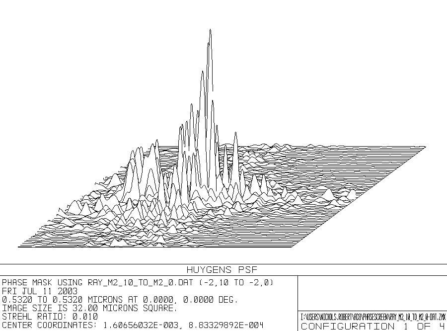
Next a phase mask was generated using a 10-meter long section perpendicular to the flow ending at a region of a high pressure gradient. This is segment "D-D" depicted in Figure 1. In this case, the propagated beam was tangent to some of the highest pressure regions of the computational data set. The Strehl ratio drops even further to a value of 0.01. As can be seen from the phase screen, the aero optics is much more complicated by this part of the flow field. The focused spot now is aberrated unsymmetrically as would be expected. Figure 5 shows the result of a beam propagating through that phase mask.
Finally, we propagate at 45 degrees to the axis of the model through the region of greatest density contours. The resulting wavefront shown in Figure 9 has a Strehl ratio of 0.083. This beam has a shorter pathlength than the other cases, being 6.4 meters.
These results show that we can interface the CFD with the aero optics code automatically. Each of these results are arrived at in seconds of run time so that an operator can run many experiments and anticipate the effects of a wide range of propagation paths and flow conditions. We have identified some apparent artifacts that arise because of our choice of grid and ray number and position.
Other Examples — We have examined many types of flow as we continue to refine the code. Some sample data are provided here as examples. Figure 10 illustrates the effect of an unsteady planar shock wave on a wavefront. The beam suffers from astigmatism, as shown in the spot diagram. The spot diagram shows where each ray in the entrance pupil ends up when focused by a perfect lens. The small circle in the center represents the diffraction limited case. With no distortion of the wavefront, all rays would fall within the circle.
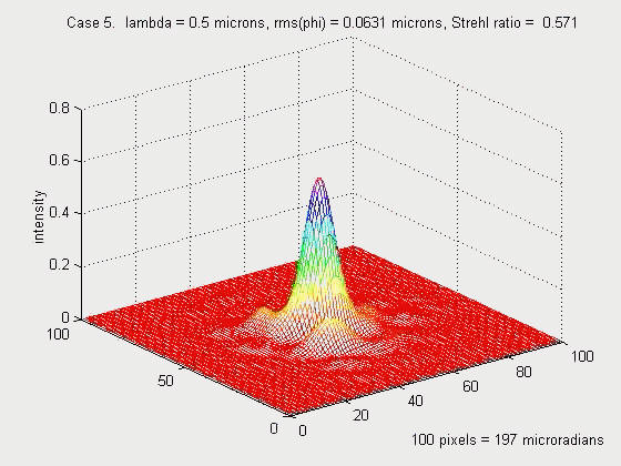
Figure 11 is an example of a point spread function of a single realization of a beam passing through a turbulent shear layer of a typical hypersonic vehicle. Many realizations can provide information about bore sight error and other useful image system parameters.
Wavelength plays an important role in aero-optics. As an example, the problem of projection from a common aircraft pod was analyzed with the AOTS code over a wide range of wavelengths. The result of the analysis is summarized in Figure 12, which plots the Strehl ratio from visible to infra red for a beam projected through the wake of the pod. In the visible, the beam suffers severe Strehl degradation, while in the infrared, aero-optics has little effect, yielding a Strehl ratio near unity.
Conclusions
The aero optics test simulator can provide systems design and test engineers with a powerful, easy-to-use tool to complement other design tools. It is intended to augment, not replace, CFD and ground testing. As more ground test and CFD data become available to aero-optics, the program will grow in capability. It provides an engineer with a method to compare and assess the importance of different aero-optical components in a flow field. It provides a first guess that can allow a test engineer to set diagnostics instrument parameters, i.e., dynamic range and sensitivity, and can help with data interpretation. It can even determine if a test is likely to be interpretable or even feasible or not. Finally, it can enable the aero-optical engineer to understand what changes can improve system performance.
 |
 |
|
Figure 1. Regions for which phase screens will be created. |
Figure 2. Aero-optics turbulence model. |
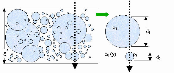
Figure 3. Turbulence model.
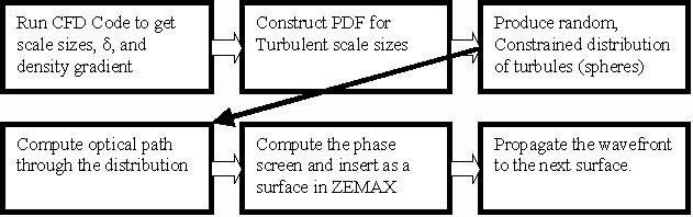
Figure 4. Algorithm for Turbulent Regions.

Figure 5. Generic turret and CFD solution showing beam paths.
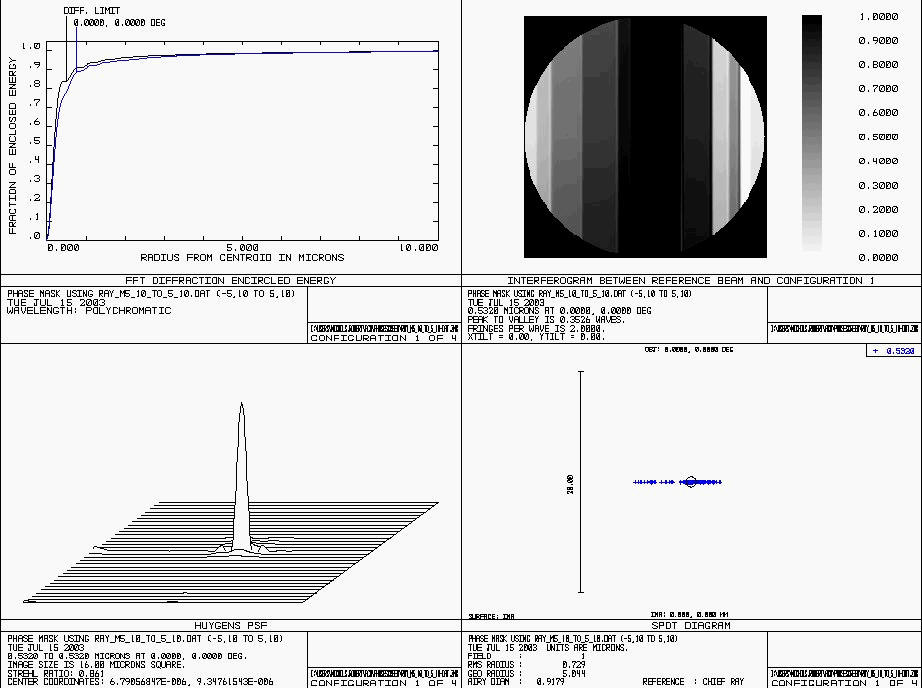
Figure 6. Composite results of propagation of a light wave in the least perturbed flow, section A-A.
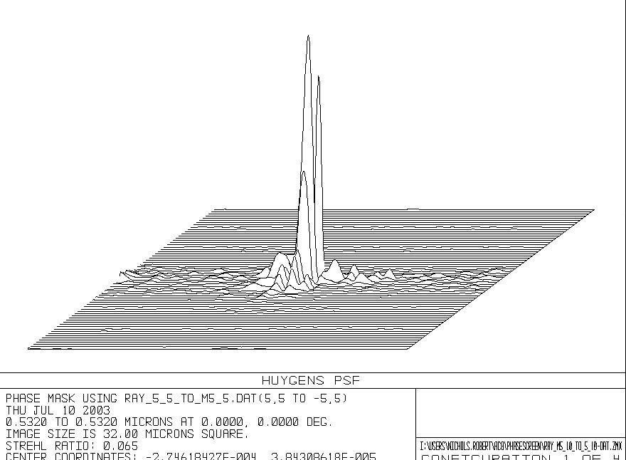
Figure 7. Results of propagation of a light wave parallel to the model axis through its flow field.
 .
.
Figure 8. Results of propagation of a light wave perpendicular to the model axis through its flow field.
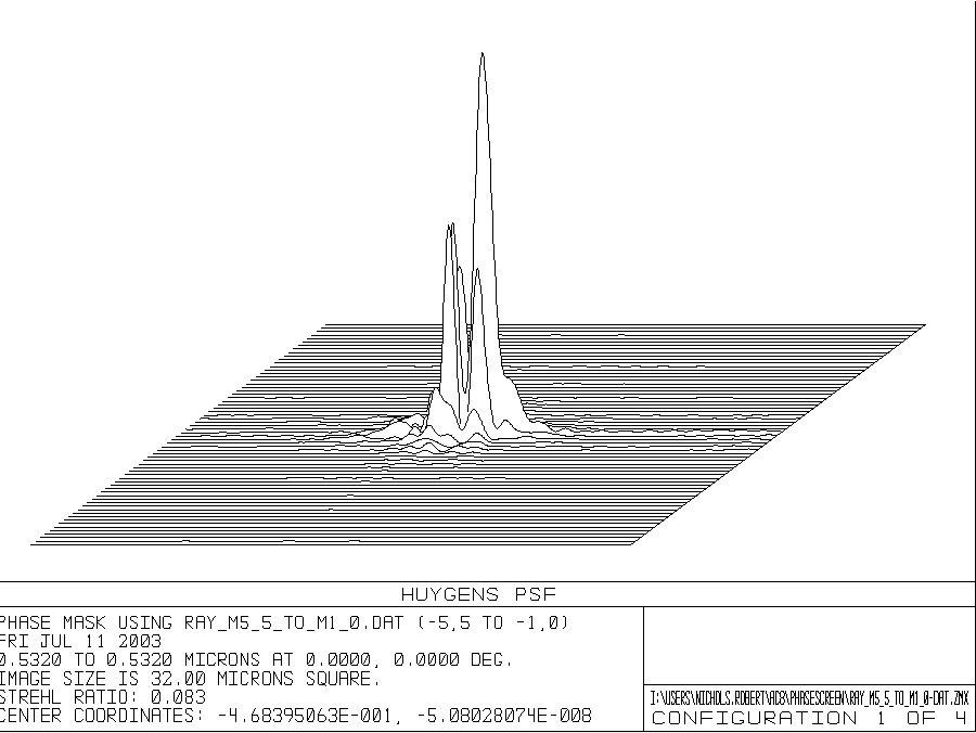
Figure 9. Results of propagation of a light wave at 45 degrees to the model axis.
 -
-
Figure 10. Aero optical effects of beam projection through an unsteady, planar shock wave.
|
|
|
|
Figure 11-Point Spread Function of a single realization through a turbulent shear layer. |
Figure 12-Strehl Ratio as a Function of Wavelength through a Turbulent Wake. |
References
[1] Trolinger, J.D., “Aero-Optical Characterization of Aircraft Optical Turrets by Holography, Interferometry, and Shadowgraph,” Aero-Optical Phenomena, Editors: Keith G. Gilbert and Leonard J. Otten, American Institute of Aeronautics and Astronautics, Inc., p. 200, (1982).
[1] J.D. Trolinger, J.E. Craig, & W.C. Rose, "Propagation Diagnostic Technique for Turbulent Transonic Flow", AIAA No. 84-0104, AIAA 22nd Aerospace Sciences Meeting, Reno, Nevada, 9-12 January 1984.
[1] Rose, W.C., and Cooley, J.M., “SOFIA Wind Tunnel Data Analysis and Implications for the Full-scale SOFIA Aircraft.”
[1] V. Lukin and B. Fortes, “Phase-correction of turbulent distortions of an optical wave propagating under conditions of strong intensity fluctuations,” Appl Optic. 41, 5616, (2002)
[1] Hinze, J.O., Turbulence: An Introduction to Its Mechanism and Theory McGraw-Hill Book Company (1959).
[1] S. Park, et al., “A study on a fast measuring technique of wavefront using a Shack-Hartmann sensor,” Optics and Laser Tech. 34, 687 (2002)
[1] Menter, F.R., “Two-Equation Eddy-Viscosity Turbulence Models for Engineering Applications,” AIAA Journal, Vol. 32, No. 8 (August 1994).
[1] Wilcox, D.C., Turbulence Modeling for CFD Second Edition. DCW Industries, Inc. (1998).
[1] James Trolinger, David Weber, and William Rose, “An Aero-optical Test and Diagnostics Simulation Technique,” presented at the AIAA International Symposium, Reno, NV, 14 January, 2002
[1] Tatom, F.B., “The Lengths and Scales of Turbulence,” Engineering Analysis, Inc., paper prepared for McDonnell Douglas Space Systems Company (September 1990).
Acknowledgements — This project is supported by an U.S. Air Force, AEDC, SBIR program. The project officers are John Lafferty and Brian Feather. The SBIR program manager is Ron Bishel.