James Trolinger

MetroLaser Incorporated

Irvine, CA 92614

This paper describes digital, photonic, two-dimensional, dynamic-wavefront sensing methods for flow diagnostics. A system described herein employs a 532 nm diode pumped solid state laser to produce quantitative, fully reduced phase maps at virtually real time acquisition rates to evaluate flows in wind tunnel facilities. This is done using instantaneous electronic phase shifting interferometry methods. Because measurements are instantaneous and not compared to a stored reference data point, the instrument is not vulnerable to vibrations and other environmental effects found in test facilities. A flow field can be analyzed quantitatively by measuring its effect on a traversing optical wavefront if the wavefront sensor can respond as fast as the field changes. Conversely, the effect of flow fields on optical imaging gives rise to the field of aero-optics, and the wavefront distortion and correction are of principal interest. Developments in aero-optics, electro-optics and image processing in general have led to more advanced variations and applications of interferometry improving speed, sensitivity, automation, and robustness. Video recording and new methods for performing high-speed interferometric wavefront and flow diagnostics electronically to speed up the process are described.

A versatile (perhaps ideal) optical instrument for flow diagnostics should incorporate features that allow the researcher to:

• record optical wavefronts with sufficient temporal and spatial resolution.

• record data at rates high enough to analyze high-speed turbulent flow.

• provide a sufficient data capacity.

• provide sufficient sensitivity and dynamic range.

• provide useful, online, near real-time flow diagnostics data.

• function in harsh wind tunnel environments.

• Install and employ the system with relative ease in a test facility.

• use it as self-contained and modular so that its components can be incorporated into existing diagnostics systems such as a Schlieren system.

• employ fiber optics to deliver the beams to the facility and for reference wave path matching for some applications.

• incorporate a rapid multiple pulsing capability to satisfy tunnel vibrational issues.

• incorporate self-calibration features.

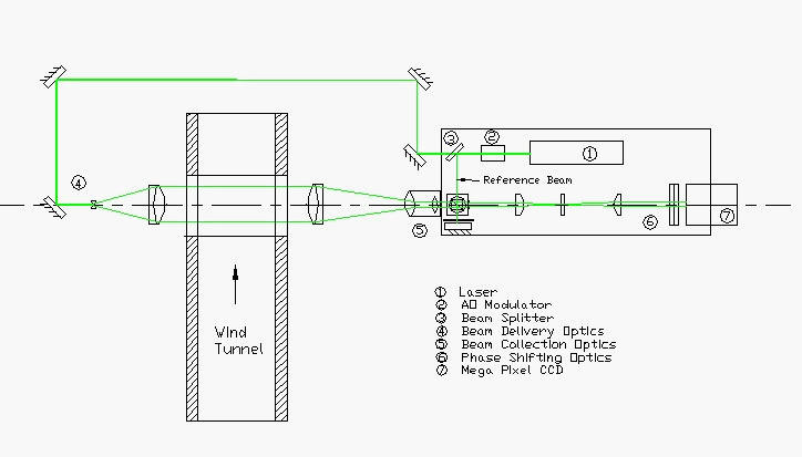
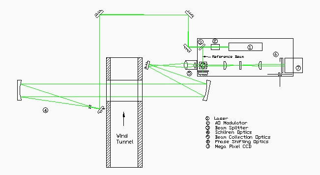
Various forms of shadowgraph, schlieren, deflectometry, and interferometry have been used for many years to analyze flow fields. As coherent and incoherent light sources, detector arrays, computers and image analysis software continue to evolve, so do the capabilities and power of all of the flow diagnostics procedures. Methods that were once cumbersome and extremely limited for many applications are becoming more and more powerful and should be re-examined for applications where they were once considered inapplicable.

Electronic imaging has allowed us to combine some of the best features of interferometry and holography leading to many improvements in capability to analyze flow fields. A crucial task of interferometry is transforming interference fringes (the interferogram) into phase or optical path length maps accurately and quickly. Of the many methods devised to accomplish this, the one that has proven most versatile and most easily adapted to video processing procedures is known as phase shifting (or stepping) interferometry^1,2. We describe here flow-measuring methods that employ instantaneous phase shifting interferometry³. The system grew out of a previously commercialized instrument termed "Phase Camâ " that was developed for the purpose of high resolution surface contouring and vibrational analysis⁴.

The fundamental system is a Mach-Zehnder interferometer enhanced by phase shifting interferometry and digital recording. Features Include:

The instrument records and produces quantitative, fully-reduced, phase maps online at high-speed in a form that can be used immediately to evaluate flows. Multiple images can be recorded with microsecond time increments and can be compared, correlated, subtracted, filtered, or saved for later processing, all electronically. This provides the versatility of holographic recording, by recording data of the same type and quality provided by conventional holographic interferometry but electronically without the use of photographic recording materials. It also meets stability and alignment requirements compatible with field application in wind tunnel facilities.

Figure 1 illustrates the basic system layout incorporating 6-inch lenses. The fundamental system can operate in other architectures illustrated in Figures 2 and 3. The system can operate with both low-cost detectors and fiber optics to achieve high-speed and spatial resolution in a robust package. The beam from a frequency doubled YAG laser (#1) is split (at beamsplitter #3) into a test object beam and a reference beam with about half of the light being conducted around the wind tunnel and being expanded into a test object beam (#4). This beam is transmitted across the test object, then collected and focused into a receiver system (#5). The receiver system focuses the collected beam and images the test section onto a phase-shifting mask (#6). Meanwhile, at beamsplitter (#3) the reference beam is conducted to a beam combining system where it is combined with the test object beam. This is achieved efficiently by passing the beam through a polarization beamsplitter and quarter wave plate where a mirror returns it to the polarization beam splitter and combines it with the test object beam. The two beams, at this stage, are now orthogonally polarized.

The beam combiner superimposes the object and reference beams and the combined beams are focused onto a diffractive optical element (DOE) that splits the combined beams into four collimated beams. The four collimated beams are identical interferograms that are passed through a quadrant phase retarder to add a discrete amount of phase difference between the object and reference waves of each interferogram. All four phase-shifted interferograms are imaged simultaneously onto a single CCD chip. A software routine then uses the four interferograms to calculate, in real-time, the phase map of the flow. By subtracting sequentially recorded images, the transient behavior of the small-scale flow structures can be recorded. In addition, images can be processed with longer time delays to record flow structures with a longer time scale. The system will provide the fast response time necessary to capture the high frequency changes found in turbulent flows.

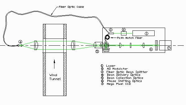
Some facilities have an excellent Schlieren system that can offer optical components that would be impractical to incorporate in a portable system. Existing Schlieren systems and those containing mirrors with an elaborate mounting system can be incorporated into the diagnostics system while retaining all of its current capabilities. Figure 2 shows how the hardware can be integrated into an existing Schlieren system. The system concept is compatible with the existing Schlieren optical hardware that is available in many test facilities.

An important breakthrough with the proposed method is that fiber optics can be used to deliver the object beam to the test section of the facility and the reference beam to the optics head. Earlier methods were not compatible with fiber optics due to a sensitivity to phase variations introduced by fibers. The proposed method solves this problem by performing the phase shifts simultaneously so that the phase of the reference wave is assured to be the same for each of the phase shifted interferograms. Implementation with fiber optics is illustrated in Figure 3. The fiber optical delivery of the beam from one side of the facility to the other would make the system more portable. Path matching requirements for the test object and reference beam must be considered here also; however, a different type of path matching is possible with fiber optics. The figure shows a fiber inserted into the reference beam for path matching.

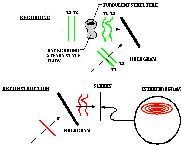
Wavefronts that traverse a transient flow can be used to analyze the time variation of the flow (Figure 4). Turbulence and other transient flow events are typically characterized by low-density (sub-fringe) events. In order to image these flow events, it is important to remove the often high-density fringes that occur due to the presence of steady-state flow. Ideally this would be accomplished by interfering two wavefronts temporally separated over a time interval in which only the transient flow features of interest change, resulting in an interference pattern that is due to those transient flow features only. Holography enables interfering two wavefronts separated in time and Time-Differential Holographic Interferometry (TDHI) has been used effectively to reveal transient flow features with high sensitivity. When two temporally separated wavefronts pass through an unsteady or turbulent flow, both wavefronts are delayed in phase an equal amount by the steady-state flow that remains unchanged during the time between wavefronts; however, the unsteady part of the flow that changes in the time between wavefronts imparts a different phase delay to each wavefront. Each wavefront is recorded electronically by interfering it with its corresponding reference wavefront at the recording plane. When photographic recording methods are employed, the exposed hologram must be processed and illuminated to reconstruct the two holographically stored wavefronts. The wavefronts, which were recorded at different times, now emerge simultaneously and interfere.

CCD cameras are now available that can record two frames with extremely short and variable time separation, precisely what is needed to achieve the time differential information. All of the reconstruction and interference are then performed in the computer, simplifying the process and reducing hardware costs significantly, as well as making the system much more reliable. It is also important to note that this technique does not require a high intensity laser source. Therefore, fiber delivery of the laser beams is possible for either CW or pulsed lasers.

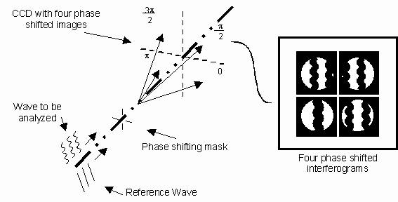
Double Exposure Imaging

Digital cameras such as the Kodak MegaPlus ES 1.0 Camera, used in this study, can capture two images in rapid succession using the triggered double exposure mode. The first image is transferred from the CCD to the frame grabber while the second image is being captured by the photo diode array. The second image is then transferred into the CCD array and then onto the frame grabber’s second image buffer. The two images can be saved as separate files.

In the Kodak camera, the time delay between the two images can be as little as 2 m s or as much as 32 ms. The timing is controlled by an external trigger pulse and a transfer pulse generated by the camera. The trigger pulse should be a 2.5V TTL pulse of at least 100 ns duration. The camera can be triggered on either the falling or rising edge of the trigger pulse. The transfer pulse delay (TPD) and transfer pulse width (TPW) are set by the user. The TPD can vary from 1 m s to 32 ms, while the TPW can vary from 1 to 5 m s. The first exposure starts 20 ± 0.1 m s after the active edge of the trigger pulse and ends on the rising edge of the transfer pulse. The second exposure begins on the falling edge of the transfer pulse and ends at the end of the camera cycle, roughly 33 ms after the initial trigger.

The triggered double exposure mode is best used in combination with illumination by a short-pulsed triggered light source such as a pulsed laser. Typically, the first light pulse is synchronized with the external trigger to the camera. The second light pulse illuminates the experiment after the transfer pulse, during the second exposure. If the time between the two light pulses is varied, the transfer pulse delay should be set to less than the minimum time delay between the two light pulses.

Interferometry is a method for determining the phase distribution over an optical wavefront by interfering the wavefront with a second well-characterized reference wavefront. The process produces interference fringes that can be analyzed to determine the difference in phase between the two wavefronts. The interference fringes in an interferogram can be described by an equation such as

I_i= I_r (x,y) + I_s (x,y) + 2[I_r(x,y) I_s(x,y) ]^0.5 X

Cos [j (x,y) + q _i], (1)

where

The equation has three unknowns, I_r, I_o, and, j (x,y), and a term, q _i that can be selected at any value by adjusting the phase of the reference wave. Of the many methods that have been devised to analyze interferograms, phase shifting interferometry (PSI) is one of the most versatile methods since it is easily adapted to take advantage of modern sensors and computers. The interferogram is presented to a CCD or similar sensor, and the term q _i is adjusted by phase shifting the reference wave, providing enough independent equations of the above form to solve for j (x,y), which is the phase difference data being sought. The solution is an inverse tangent function of the intensities, I_i.

A method based on the instantaneous phase measurement technique developed by Smythe and Moore⁵ for generating multiple phase-shifted images simultaneously, is illustrated in Figure 5. The procedure developed in this work employs a Holographic Optical Element (HOE) and a quadrant phase retardation mask to produce a compact, single CCD camera system^6,7 This method produces four phase-shifted interferograms that are imaged onto a CCD camera. The waves are matched in such a way that the CCD (even with low resolution) is adequate for directly recording sufficient information for flow diagnostics. This particular phase shifting procedure eliminates the usual problem encountered with the use of fiber optics for interferometry. Fibers are extremely sensitive to temperature and will add phase errors when conventional methods are employed; however, the procedure described here subtracts these errors in the final process.

(2)

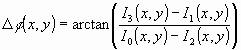
For most applications, a change in the phase map is the quantity of greatest interest. Therefore, subtraction procedures should enable the removal of constant terms, such as system optics effects. These procedures, which have represented one of the greatest benefits of holographic interferometry, are even easier to implement electronically and off additional advantages. Subtracting two phase maps can eliminate constant noise terms. The method applies to the comparison of a flow field with some reference baseline or to the flow field at two different times (e.g. the diagnostics of turbulence). To determine absolute quantities, a baseline interferogram of the stationary field is first captured to provide a record that contains invariant system information. Subtraction of this baseline interferogram from that of the data wave leaves only information representing changes in the wavefront. A unique phase difference algorithm allows wavefronts to be compared efficiently and accurately⁸, and also helps with noise cancellation and management. By solving for phase differences directly, the number of inverse tangent operations can be cut in half. The process can be speeded up even more if the amplitudes of the object and reference wavefronts remain constant. With this assumption they can be measured once, then equation 1 has only one variable and can be solved with no additional phase shifts. If the amplitudes do not change between two measurement times, then the phase difference between the two conditions can be solved with only one phase shift, even without measuring the amplitudes. These kinds of possibilities lead a wide variety of system optimizations for different types of applications.

Flow structures characterized by different length (time) scales can be isolated by recording interferograms at variable time separations. Subtraction of the processed phase maps with a time delay of D t, in effect, records the flow structures with the characteristic time scale D t. Features that do no vary within this time are eliminated. Phase difference maps provide a variety of useful information. The baseline can be a no-flow case or it can be a flow case taken at a different time. Comparison with a no-flow case leads to absolute flow field data, which represents the steady flow field plus the unsteady field, while comparisons with other flow fields can characterize the time changes in the flow, which represent the unsteady flow.

To look at high-speed events requires either a pulsed laser or some other form of fast shuttering with a CW laser. For data presented here we added an acousto-optic modulator for time gating of the continuous laser beam.

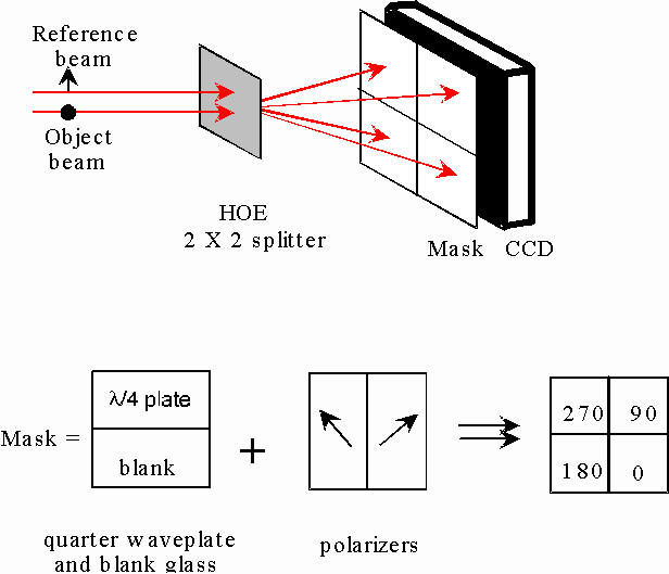
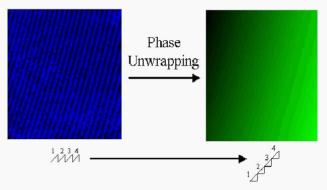
Figure 5. Wavefront analyzer.

In PSI there exists an ambiguity in the solution for phase for each increase by 2P . Therefore, the reduced interferogram first appears as a discontinuous function, called the ‘wrapped’ phase map. The wrapped phase map does not distinguish an increase from a decrease in phase in each cycle when the wave varies by more than one wavelength. To get the final answer requires unwrapping of the phase map. Figure 6 and Figure 7 are examples of wrapped and unwrapped phase maps. The image on the left is the ‘wrapped’ phase map, obtained from the set of four phase-shifted interferograms. In this phase map, each bright-dark-bright fringe represents a 2p change in the optical phase, which is directly proportional to an optical path length change of one wavelength. The image on the right is the ‘unwrapped’ phase map, in which the 2p ambiguities have been resolved. By using information from all four phase-shifted interferograms, the ambiguities at 2p phase jumps can be properly resolved.

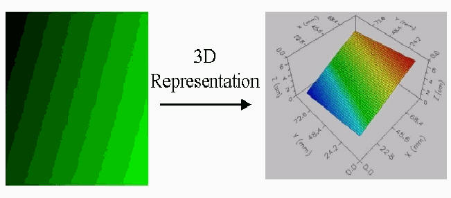
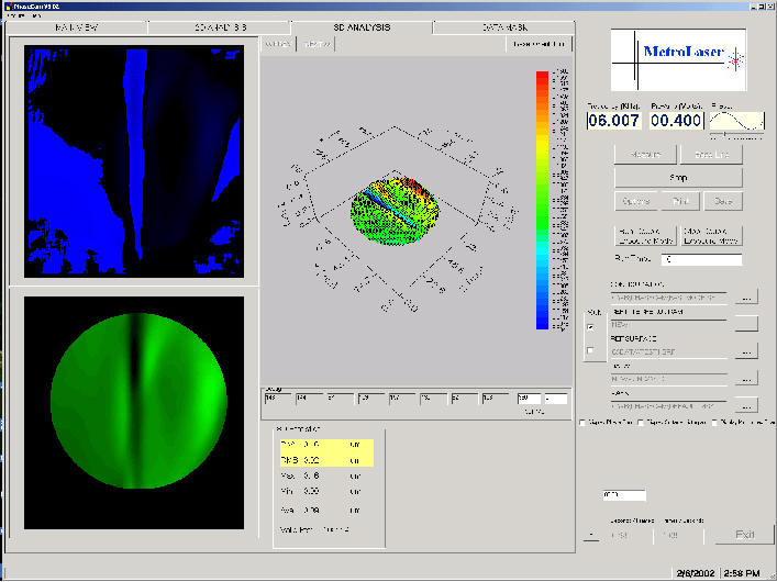
It is important here to distinguish between interferograms and phase maps. It is also important to emphasize that a phase map is much more than an interferogram since it is the result of an analysis of the interferogram, and actually contains all of the information processed from four interferograms. An interferogram is a contour map of phase and has the problem that phase is still encoded in sinusoids so it cannot be read directly and is difficult to interpret. A wrapped phase map is also a contour map but has much better contrast than its interferogram, it is linearized with density, and it can be much more useful even before it is unwrapped. The unwrapped phase map is actually a picture of the wavefront in 3-D.

A self-calibration procedure developed for this system comprises a controllable mirror that acts as a phase object simply by adding a known amount of tilt. Tilting the wavefront under study adds a wedge phase object of known optical path length in the system. We use this tilt to confirm the accuracy and the sensitivity of the measured phase map. The procedure also allows other useful assessment of the data.

Figure 6 illustrates the phase map of a wavefront that is tilted by about 30 waves across the field-of-view. The image on the left is the ‘wrapped’ phase map, obtained from a set of four simultaneous phase-shifted interferograms. In this phase map, each bright-dark-bright fringe represents a 2p change in the optical phase, which is directly proportional to an optical path length change of one wavelength. The image on the right is the ‘unwrapped’ phase map, in which the 2p ambiguities have been resolved. By using all of the information collected in the procedure, the ambiguities at 2p phase jumps can be properly resolved. Figure 7 shows the resulting quantitative gray scale map and its associated 3-D representation. The spatial position is shown on the x and y axes, and the height is shown on the z-axis. In this example, the wavefront was tilted approximately 15 microns.

To illustrate the system capability, we created various turbulent flows with features like those encountered in wind tunnel studies, though much slower⁹. The examples shown here are for slow moving flow fields generated by heat guns, flames, and low velocity air jets. We made a wide range of measurement on these flow fields to test the various measurement concepts using the system. We were able to test the system in all of the desired modes with these simple flow fields. We also demonstrated the spectral analysis capability of the system, adjusting the time delay between recordings to show different flow features.

The output of the system comprises a phase map, which is a reduced interferogram. This is not to be confused with the interferogram itself, which is actually raw data, and without further processing provides only a qualitative look at the flow field, simply, a flow visualization picture. The phase map incorporates all of the data from four simultaneously recorded interferograms and quantifies the flow field, essentially in real-time. This provides the quantitative measure of the optical path length change caused by the flow field. It comprises a line integral of the density along the view path through the flow field.

Flow diagnostics entails measuring density changes as a function of time and position. This is achieved with the present system by recording a reference (i.e., initial condition) frame and subsequent measurement frames. If the reference is a no flow condition, then the path difference between the "measurement" and the "reference" represents the effect of the entire absolute flow field, the steady plus unsteady flow with all constant window and optical effects removed. On the other hand, if the flow field itself at time t₁ is used as a reference condition while the "measurement" frame corresponds to the flow field at time t₂, then the resulting phase difference map is a quantitative measure of the change in density of the flow field with time. Not only are all constant window and optical effects removed, but also steady flow effects, such as laminar flow, are removed providing a measure of the unsteady effects, that is, the turbulent flow. By comparing two recordings with variable time spacing, one can in fact, analyze the spatial-temporal nature of the turbulence.

To convert optical path differences to point density requires either more knowledge about the geometry of the flow field or additional views through the flow field. If the density has a known distribution across the flow field, then the point density is determinable from this single view. If no symmetry exists, then multiple views and tomography are required to transform the projection into the 3-D density function.

The flow fields shown here include both laminar and turbulent flow to demonstrate the concept. The objective of these examples is to illustrate that the method is capable of producing high-speed movies of quantitative flow field profiles computed from the recorded wavefronts. An electrically controllable heater produced a free convective flow. The flow begins as laminar and goes turbulent as the Reynolds number increases during its rise from the heater, producing fairly regular vortices for testing the diagnostics procedure. Figure 8 illustrates a typical display with the present setup. The output screen of the instrument provides the wrapped phase map (upper left), the unwrapped phase map (lower left), and the 3-D display (center).

The system can be operated in various modes, depending on the specific experiment. For example, interferograms appearing on the CCD can be collected by a frame grabber and then dumped to memory (four phase-shifted interferograms for each stored CCD frame). In this system, the storage rate is 15 per second, or 0.066 seconds between stored recordings when using conventional video rate cameras. This limitation is a result of the particular frame grabber and computer combination. The recording speed can be easily increased by using high-speed cameras to record the interferograms or by using the double exposure method available with some CCD cameras. This could reduce the time between recordings to the m s range. Another method to increase recording time is to employ two CCD cameras that record the same field-of-view (through a beamsplitter) at slightly different times.

Quantitative density information is subsequently obtained by transforming the information stored in the phase maps, which provide quantified optical path length changes. We give here an example computation of a density change in a turbulent flow. Since each frame captures four phase-shifted images to determine phase difference between two stored frames, all eight phase-shifted images are used to determine the phase difference to be computed with one inverse tangent operation. The entire operation takes a fraction of a

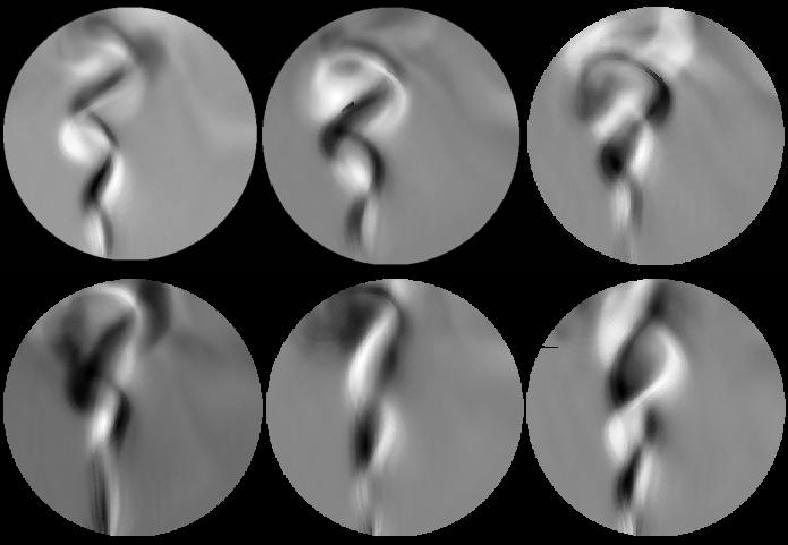
second for each image pair. This includes obtaining the solution in the so-called "wrapped" form where a 2P ambiguity exists for each place the path length increases or decreases by one wavelength. Finally, the phase is then unwrapped, and the optical path length change is displayed.

Figure 9 shows six phase difference maps, recorded in time sequence with approximately 0.06 seconds between recordings, using the flow field itself as a reference. Each flow field is referenced to the previous flow field of 0.06 seconds earlier. We made the flow slow enough to allow correlation between the recordings. (These time separations can be decreased arbitrarily with the right hardware.)A number of observations can be made with these data. Note how clear and noise free the background appears. The unperturbed region outside the flow field does not change between the two recordings. Therefore, one may expect this to appear black in the phase difference map. The level of the background has been adjusted to accommodate negative phase information. The lowest value of phase is set to zero (or black), therefore the background is gray.

The phase difference map looks remarkably like a white light Schlieren presentation of the flow. The similarity is not an accident of course, since Schlieren maps gradients in the density of a flow field. Here we have the added feature that the intensity is directly proportional to the phase difference. Since the temperature and pressure are relatively constant in this flow, the path length change is caused by geometrical changes in the flow field that take place in the time between recordings. The flow clearly has a "corkscrew-like" appearance. As the flow rises, the corkscrew moves upwards and the path length through it changes. With these assumptions, one can actually quantify this flow field as it develops in time.

From this data, we can determine that the change in optical path difference between the regions of maximum decrease and increase in temperature is about 0.6 m m, or ± 0.3 m m relative to the background (where conditions are assumed to be constant). Thus, between frames the average refractive index changes from the ambient value, D n say, through these regions are given by

.

Taking a value for the Gladstone-Dale constant of 2.25x10^-4 m³ kg^-1, we find the average change in density to be

kg m^-3.

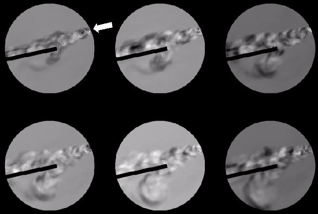
The density of air at 15° C is approximately 1.3 kg m^-3, so the relative change is about ± 0.08 percent.

This, of course, is a simplified example. A detailed and accurate 3-D flow map requires a detailed knowledge of the flow geometry. One-dimensional flows and axisymmetric flows can be analyzed with a single view. More complex views without additional knowledge require at least four different angular views through the flow to be used together with tomographic analysis. Otherwise, the quantities represent an average density change along the line of sight.

Another flow field that we used for system development is a gas jet flow (shown in Figure 10), again maintained at low velocity to accommodate our current low recording rate. The flow is split by a plate to make it more representative of a wind tunnel flow of interest. Again, note the clean, noise-free background. One only has to compare this with the typical holographic interferogram to fully appreciate the power of the technique. Here we track the progression of a vortex across the field-of-view. Again, these are quantitative results. And the images allow us to monitor extremely small changes in the flow field associated with the unsteady part of the flow. They measure the change in optical path length that took place in the time between recordings, allowing us to subtract noise and steady flow effects. With some assumptions we can derive the velocity and other turbulence parameters in this flow.

The digital, photonic, flow diagnostics system, described here should find wide spread application in flow diagnostics. It captures all of the power of time tested optical diagnostics tools in a way that will allow it to be installed and used more easily, while providing on line quantitative data in near real time. The quality of the data can actually excel over that of film recording systems because electronic processing allows for direct subtraction of noise generating amplitude and phase elements in the system in addition to versatile image processing tools. We anticipate this to represent a new class of flow diagnostics tools that will eventually replace methods that use photographic materials.

REFERENCES